🎧 Sampling and Quantization Explained

Welcome back to Hobitronics, your go-to space for demystifying electronics and communication concepts with clarity and creativity. Today, we begin a fundamental journey through how analog signals become digital, forming the bedrock of everything from your voice call to digital music and embedded sensor systems.

We’ll dive deep into the two most critical steps: Sampling and Quantization. These processes are essential for converting real-world continuous signals into digital data that machines can store, process, and transmit.

🌊 The Real-World is Analog

Most physical phenomena—sound, light, temperature, voltage—are analog in nature. This means they vary smoothly and continuously over time. But computers, microcontrollers, and communication systems operate in the digital domain—they understand only discrete values, especially binary (0s and 1s).

So how do we bridge this analog-digital divide?

By converting analog signals into digital ones using Analog-to-Digital Conversion (ADC), a process that mainly involves:

1. Sampling — capturing the signal at regular time intervals

2. Quantization — assigning those samples to discrete amplitude levels

Let’s understand both in depth.

🎚️ 1. Sampling — Taking Snapshots in Time

🔍 What is Sampling?

Sampling is the process of measuring the value of an analog signal at uniform time intervals.

You can think of it like recording a video. A camera takes 30 or 60 frames per second to create a sense of continuous motion. Similarly, sampling takes a "snapshot" of the analog signal at fixed intervals.

🧠 Why Sample?

You can’t store or process infinite values. So instead of recording every microsecond of a signal, we sample it periodically. This gives us a discrete-time representation of the signal—values only at certain moments, not continuously.

📏 Sampling Rate (Fs)

This is the number of samples taken per second, measured in Hertz (Hz).

For example:

• Fs = 1000 Hz → 1000 samples taken per second

• Fs = 44100 Hz → CD-quality audio sampling

The sampling rate directly impacts how accurately we can represent the original analog signal.

🎯 The Nyquist-Shannon Sampling Theorem

This famous theorem tells us:

To avoid losing information, the sampling rate must be at least twice the highest frequency present in the analog signal.

This critical value is called the Nyquist Rate.

Example:

If you’re digitizing an audio signal with max frequency 20 kHz:

• You must sample at Fs ≥ 40 kHz

• That’s why CD audio is sampled at 44.1 kHz

⚠️ What Happens if You Under sample?

If your sampling rate is too low, you get aliasing — a form of distortion where different signals become indistinguishable.

Imagine a spinning wheel that looks like it's going backward on camera — that's aliasing in action.

To avoid this, anti-aliasing filters are often used before sampling to remove high-frequency components.

🧮 2. Quantization — Freezing Amplitude into Levels

Now we’ve got sampled values—great! But they’re still analog voltages, like 2.75 V, 1.94 V, etc. Computers can’t directly store or manipulate real-world voltages—they need numbers.

That’s where Quantization comes in.

🔧 What is Quantization?

Quantization is the process of rounding each sampled value to the nearest discrete level from a fixed set. This set is determined by how many bits we use to represent each sample.

So now:

• Time is discrete (due to sampling)

• Amplitude is also discrete (due to quantization)

We’ve transformed a smooth, continuous signal into a discrete-time, discrete-amplitude signal — perfect for digital systems!

🔢 Bit Depth and Quantization Levels

The bit depth determines how many quantization levels you can have:

• More bits = higher precision

• Fewer bits = more quantization error, but lower data size

Example:

If your voltage range is 0V to 5V and you use 8 bits (256 levels), each level represents:

Δ = (5V - 0V)/256 ≈ 0.0195 V

So any measured voltage gets rounded to the nearest multiple of 0.0195V.

🤖 Quantization Error and Noise

Quantization introduces a round-off error, known as quantization noise. This is the difference between the actual sampled value and its quantized representation.

While small, in high-precision systems like medical imaging or radar, this error can be critical. That’s why such systems use higher bit depths.

To minimize this error:

• Use more bits (finer resolution)

• Use techniques like dithering to spread error uniformly

🔌 Real-World Example: ADC in Action

Let’s say we want to digitize a voice signal:

• Human speech ranges from 300 Hz to 3400 Hz

• Sampling rate chosen: 8000 Hz (satisfies Nyquist)

• Quantization: 8-bit (256 levels)

Each second of speech produces:

• 8000 samples × 8 bits = 64,000 bits = 8 KB

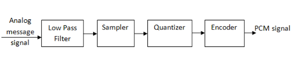
This is the basis for Pulse Code Modulation (PCM), used in traditional telephony — and the topic for your next blog!

🎯 Final Thoughts

Understanding Sampling and Quantization gives you a strong foundation in digital signal processing, embedded systems, audio engineering, and telecommunications.

Every sound you hear from your phone, every ECG signal from a heart monitor, every sensor reading in an IoT system — they all depend on these two steps.

In our next Hobitronics blog, we’ll build on this and explore:

• Encoding methods

• PCM (Pulse Code Modulation) structure

• How signals are finally converted into 0s and 1s for computers and communication

Stay tuned, and if you enjoyed this, do share it with your fellow learners! 🚀For more such awesome, techy, and easy-to-understand blogs on cutting-edge innovations, practical electronics, and the future of communication systems stay tuned to hobitronics.blog!